Dynamic MuJoCo Model and Simulation

This page documents how the ArcFold inchworm-inspired foldable robot is converted from the Assignment 1 kinematic concept into a dynamic MuJoCo model with compliance, actuators, and performance tracking, as required for Project Assignment 2. The same model is used to study how gait timing (period) influences the achievable speed and robustness of the Sarrus‑linkage inchworm crawler, in parallel with experiments on the physical prototype.

1.1 Robot Overview and Objectives

The ArcFold robot is a planar Sarrus‑linkage inchworm crawler with two friction‑modulated pads and a central body that retracts and extends to realize a lift–drag gait. The simulated geometry is consistent with the laminated triangular body and two‑pad layout described in the Design section of the project.

Biological inspiration. The mechanism abstracts the looping, two‑anchor gait of Manduca sexta: the rear pad anchors while the body arches and the front pad advances; then the front pad anchors while the rear pad is pulled forward.
Model objectives. The MuJoCo model is constructed to
- capture the robot’s planar dynamics (forward translation and arching),
- include joint stiffness, joint damping, and servo‑like actuator dynamics informed by Assignment 5 parameter identification, and
- provide a reproducible platform for sweeping gait period and comparing simulation results directly with hardware experiments.

1.2 Model Structure: Bodies, Joints, and Contacts

The MuJoCo model represents the ArcFold mechanism as a small set of rigid bodies connected by hinge joints and constrained into a Sarrus‑like spatial linkage. The key elements are:

Rigid bodies
- foot1 – front pad that can pivot to increase or decrease contact with the substrate.
- foot2 – rear pad with analogous functionality at the tail.
- first_left, second_left, first_right, second_right – central body segments that form the two mirrored Sarrus legs.
- base_bot, base_left, base_right, tail_left, tail_right, tail_bot – base and tail segments that close the linkage loop and approximate the folded triangular body of the physical robot.
- end_effector – small tracking body located near the front of the robot and used for performance sensing.
Joints
- first_left, first_right, last_left, last_right – outer hinges of the Sarrus linkage.
- mid_left, mid_right – central arching hinges, modeled as compliant joints.
- foot1, foot2 – pad pivot joints that control pad contact angle with respect to the body.
Contacts and friction
- All rigid bodies interact with a single ground plane geom ground.
- Pad geoms associated with foot1 and foot2 use friction parameters based on the tape‑foot material, while base geoms use friction parameters based on the laminated body material.
- During the gait, friction modulation is achieved by shifting normal load between pad and body geoms through coordinated rotation of the pad joints and central body.

A concise summary of the main model elements is given in Table 1.

Element type	Name(s)	Description
body	`first_left`, `first_right`, `second_left`, `second_right`	Central body segments
body	`foot1`	Front pad body
body	`foot2`	Rear pad body
joint	`mid_left`, `mid_right`	Main arching hinges (compliant)
joint	`foot1`	Front pad pivot
joint	`foot2`	Rear pad pivot
body	`end_effector`	COM / performance tracking site
geom	`ground`	Ground plane

1.3 Compliance and Actuator Modeling

The dynamic model includes both structural compliance at the laminated flexure joints and simplified actuator dynamics for the servo‑driven joints.

Joint compliance
The flexure hinges in the physical ArcFold robot are represented as torsional springs and dampers on the model joints (first_left, first_right, mid_left, mid_right, last_left, last_right). In the XML template, these appear as stiffness="{k_joint}" and damping="{b_joint}". The parameters
- torsional stiffness \(k_\theta\), and
- torsional damping \(b_\theta\),
are taken from the Assignment 5 parameter‑identification experiments on the laminated hinge material and applied uniformly to all modeled flexure joints.
Actuator model
Joint actuation is modeled using MuJoCo position actuators attached to
- the central Sarrus hinge (mid_act acting on joint mid_left), and
- the front and rear pad pivots (actuators foot1 and foot2 acting on joints foot1 and foot2).
Each actuator uses two gains:
- proportional gain \(k_p = k_{\text{motor}}\), which sets an effective rotational stiffness between the joint angle and the commanded target angle, and
- derivative gain \(k_v = b_{\text{motor}}\), which adds velocity‑proportional damping.
The numerical values of \(k_{\text{motor}}\) and \(b_{\text{motor}}\) are drawn from servo‑fitting based on RC servo data and remain approximate; the current model therefore captures qualitative servo behavior but not full torque and velocity limits.
The control inputs supplied from Python are joint target angles given by periodic square‑wave functions of time. The amplitudes and relative phase offsets of these waves define the gait timing: the feet alternate between anchored and lifted configurations while the central hinge alternates between compressed and extended states.
Friction model and friction modulation
Distinct friction parameters are assigned to pad and body geoms via MuJoCo’s friction attribute:
- pad geoms use \(\mu_\text{tape}\), measured for the tape‑based pad material, and
- base geoms use \(\mu_\text{base}\), measured for the laminated body on the test surface.
These coefficients are imported from the Assignment 5 friction experiment. Because the pads and body experience different normal loads over the gait cycle, the combination of different \(\mu\) values and changing normal force realizes friction modulation: during anchoring phases most of the normal load is carried by the active pad, whereas during swing phases that pad is rotated to reduce contact while the opposite pad or body carries more of the load.

1.4 Sensing and Performance Metric Definition

The MuJoCo model includes a dedicated body end_effector near the front of the robot. A small spherical geom is attached to this body and used purely for sensing and visualization.

Spatial sensing
During simulation, the global position data.body('end_effector').xpos is logged at a fixed sampling rate. Its x‑coordinate provides a direct measure of forward progress of the crawler on the ground plane.
Performance metric
The primary scalar performance metric is forward displacement in the x‑direction over the simulation window: \(\Delta x = x_{\text{end}}(t_\text{final}) - x_{\text{end}}(t_0).\)
For a given gait period \(T_\text{gait}\), an average forward speed is estimated as \(v \approx \frac{\Delta x}{t_\text{final} - t_0},\) consistent with the definition used in the overall project description. For the timing study, \(\Delta x\) and \(v\) are computed for several gait periods (4 s, 2 s, 1 s, 0.5 s) so that performance in simulation can be compared directly to the tracked motion of the physical ArcFold robot.

1.5 MuJoCo XML Template

The MuJoCo model is instantiated from a Python string template. Placeholder fields such as {k_joint}, {b_joint}, {mu_tape}, {mu_base}, {mass}, {k_motor}, and {b_motor} are filled in at run time from experimentally identified parameters or design choices. This approach allows the same XML structure to be reused while sweeping over friction, compliance, actuator gains, or mass properties.

Structurally, the template defines:

a ground plane geom ground,
base and tail bodies (base_*, tail_*) that form the triangular ArcFold body,
the left and right Sarrus legs built from first_* and second_* body segments,
pad bodies foot1 and foot2 with their own contact geoms and hinges,
weld equality constraints that close the Sarrus linkage, and
three position actuators that drive the central hinge and both pad pivots.

The Python and XML template used in the notebook are shown below.

import os
import mujoco
import pandas
import numpy as np
import math
import mediapy as media
import matplotlib.pyplot as plt
import imageio_ffmpeg
from scipy import signal

# ---------------------------------------------------------------------------
# MuJoCo XML template for the ArcFold Sarrus-linkage inchworm crawler
#
# This template is filled from Python with:
#   mu_base : friction coefficient for low-friction base/structural contacts
#   mu_tape : friction coefficient for high-friction pads (anchor contacts)
#   mass    : link mass for each Sarrus linkage segment
#   k_joint : torsional stiffness of flexure joints (structural compliance)
#   b_joint : torsional damping of flexure joints
#   k_motor : position actuator proportional gain (servo stiffness)
#   b_motor : position actuator derivative gain (servo damping)
#
# Units:
#   length  -> meters
#   mass    -> kilograms
#   time    -> seconds
#   gravity -> m/s^2
#
# The model consists of:
#   - A bottom base body with an attached front pad (foot1)
#   - Left and right Sarrus-linkage chains that create the arching motion
#   - A rear base body with an attached rear pad (foot2)
#   - Weld constraints tying the left/right chains together (parallel mechanism)
#   - Position actuators driving the central hinge and both feet
# ---------------------------------------------------------------------------

xml_template = '''
<mujoco>
    <default>
        <!-- Simple lighting and camera defaults -->
        <light castshadow="false" diffuse="1 1 1"/>
        <camera fovy="45"/>
    </default>

    <!--
    Global simulation options:
      - RK4 integrator for improved stability
      - Small timestep for contact-rich inchworm dynamics
      - Standard Earth gravity along -z
    -->
    <!--<option><flag contact="disable"/></option>-->
    <option integrator="RK4"/>
    <option timestep="1e-4"/>
    <option gravity="0 0 -9.81"/>

    <worldbody>
        <!-- Overhead lights for even illumination along the crawl direction -->
        <light name="top"  pos="0 0 2"/>
        <light name="top1" pos="1 0 2"/>
        <light name="top2" pos="2 0 2"/>
        <light name="top3" pos="3 0 2"/>
        <light name="top4" pos="4 0 2"/>

        <!-- Camera views used for debug videos and qualitative inspection -->
        <camera name="triangle" pos="7 0 .75"  euler="90 90 0"/>
        <camera name="triangle2" pos="-2 0 .05" euler="90 -90 0"/>
        <camera name="iso"    pos="-2 -3 3"    euler="45 -45 -30"/>
        <camera name="iso2"   pos="10 -6 6"    euler="45 45 30"/>

        <!-- Flat ground plane; contype/conaffinity define contact bitmasks -->
        <geom name="ground" type="plane" pos="0 0 -.25" size="15 15 .05"
              rgba=".5 .5 .5 1" contype="2" conaffinity="1"/>

        <!--
        FRONT MODULE (base_bot):
          - Free-flying base box that carries the front pad (foot1)
          - Uses low friction (mu_base) when the body itself contacts the ground
        -->
        <body name="base_bot" pos="0 0 0">
            <!-- 6-DOF base joint (translation + rotation) -->
            <joint type="free"/>

            <!-- Front base body -->
            <geom type="box" size=".5 .5 .05" pos=".5 0 0"
                  rgba="1 0 0 .25" mass=".1"
                  contype="1" conaffinity="1"
                  friction="{mu_base} 0.0 0.0"/>

            <!-- Front pad (foot1) providing high-friction anchoring -->
            <body name="foot1" pos="0 0 0">
                 <geom type="box" size=".1 .25 .05" pos=".15 0 0"
                       rgba="0 1 0 1" mass=".1"
                       contype="1" conaffinity="1"
                       friction="{mu_tape} 0.0 0.0"/>
                 <!-- Hinge joint for front pad pitch (used by foot actuator) -->
                 <joint name="foot1" type="hinge" axis="1 0 0" pos=".25 0 0"/>
            </body>
        </body>

        <!--
        LEFT SARRUS CHAIN:
          - base_left, first_left, second_left, tail_left form one side of the Sarrus linkage
          - Each hinge has torsional stiffness/damping representing flexure joints
        -->
        <body name="base_left" pos="0 .25 .433" quat=".866 -.5 0 0">
            <joint type="free"/>

            <!-- Left front base segment -->
            <geom type="box" size=".5 .5 .05" pos=".5 0 0"
                  rgba="1 0 0 .15" mass="{mass}"
                  contype="1" conaffinity="1"/>

            <!-- First left link -->
            <body name="first_left" pos="1 0 0" axisangle="0 1 0 -45">
                <!-- Flexure hinge at first left joint -->
                <joint name="first_left" type="hinge" axis="0 1 0" pos="0 0 0"
                       range="-45 45" stiffness="{k_joint}" damping="{b_joint}"/>
                <geom type="box" size=".5 .5 .05" pos=".5 0 0"
                      rgba="1 1 1 .25" mass="{mass}"
                      contype="1" conaffinity="1"/>

                <!-- Second left link -->
                <body name="second_left" pos="1 0 0" axisangle="0 1 0 90">
                    <!-- Central Sarrus hinge on left side (arched motion) -->
                    <joint name="mid_left" type="hinge" axis="0 1 0" pos="0 0 0"
                           range="-90 90" stiffness="{k_joint}" damping="{b_joint}"/>
                    <geom type="box" size=".5 .5 .05" pos=".5 0 0"
                          rgba=".5 .5 .5 .25" mass="{mass}"
                          contype="1" conaffinity="1"/>

                    <!-- Tail left link -->
                    <body name="tail_left" pos="1 0 0" axisangle="0 1 0 -45">
                        <!-- Rear flexure hinge on left side -->
                        <joint name="last_left" type="hinge" axis="0 1 0" pos="0 0 0"
                               range="-45 45" stiffness="{k_joint}" damping="{b_joint}"/>
                        <geom type="box" size=".5 .5 .05" pos=".5 0 0"
                              rgba="1 0 0 .25" mass="{mass}"
                              contype="1" conaffinity="1"/>

                        <!--
                        REAR MODULE (tail_bot) & rear pad (foot2):
                          - tail_bot: rear base box, low friction (mu_base)
                          - foot2: rear pad, high friction (mu_tape)
                        -->
                        <body name="tail_bot" pos="0 .25 -.433">
                            <geom type="box" size=".5 .5 .05" pos=".5 0 0"
                                  rgba="1 0 0 .25" mass=".1"
                                  quat=".866 .5 0 0"
                                  friction="{mu_base} 0.0 0.0"
                                  contype="1" conaffinity="1"/>

                            <!-- Site near the rear "head" used as end-effector tracking point -->
                            <body name="end_effector" pos="1 -.375 .2165">
                                <geom type="sphere" size=".1" pos="0 0 0"
                                      rgba="1 1 1 1" mass=".00001"
                                      contype="1" conaffinity="1"/>
                            </body>

                            <!-- Rear pad (foot2) with its own hinge and high friction -->
                            <body name="foot2" pos="0 -.25 -.433" quat=".866 .5 0 0">
                                <!-- Hinge joint for rear pad pitch (used by foot actuator) -->
                                <joint name="foot2" type="hinge" axis="1 0 0" pos=".55 .5 0"/>
                                <geom type="box" size=".1 .25 .05" pos=".75 .5 0"
                                      rgba="0 1 0 1" mass=".1"
                                      contype="1" conaffinity="1"
                                      friction="{mu_tape} 0.0 0.0"/>
                            </body>
                        </body>
                    </body>
                </body>
            </body>
        </body>

        <!--
        RIGHT SARRUS CHAIN:
          - Mirrors the left chain; welded together in the equality section to form a 3D Sarrus linkage
        -->
        <body name="base_right" pos="0 -.25 .433" quat=".866 .5 0 0">
            <joint type="free"/>

            <geom type="box" size=".5 .5 .05" pos=".5 0 0"
                  rgba="1 0 0 .25" mass="{mass}"
                  contype="1" conaffinity="1"/>

            <body name="first_right" pos="1 0 0" axisangle="0 1 0 -45">
                <joint name="first_right" type="hinge" axis="0 1 0" pos="0 0 0"
                       range="-45 45" stiffness="{k_joint}" damping="{b_joint}"/>
                <geom type="box" size=".5 .5 .05" pos=".5 0 0"
                      rgba="1 1 1 .25" mass="{mass}"
                      contype="1" conaffinity="1"/>

                <body name="second_right" pos="1 0 0" axisangle="0 1 0 90">
                    <joint name="mid_right" type="hinge" axis="0 1 0" pos="0 0 0"
                           range="-90 90" stiffness="{k_joint}" damping="{b_joint}"/>
                    <geom type="box" size=".5 .5 .05" pos=".5 0 0"
                          rgba=".5 .5 .5 .25" mass="{mass}"
                          contype="1" conaffinity="1"/>

                    <body name="tail_right" pos="1 0 0" axisangle="0 1 0 -45">
                        <joint name="last_right" type="hinge" axis="0 1 0" pos="0 0 0"
                               range="-45 45" stiffness="{k_joint}" damping="{b_joint}"/>
                        <geom type="box" size=".5 .5 .05" pos=".5 0 0"
                              rgba="1 0 0 .25" mass="{mass}"
                              contype="1" conaffinity="1"/>
                    </body>
                </body>
            </body>
        </body>
    </worldbody>

    <!--
    Equality constraints:
      - Weld left/right bases and tails so the two chains act as a single Sarrus linkage.
      - This enforces the parallel-mechanism behavior used in the ArcFold robot.
    -->
    <equality>
        <weld body1="tail_bot"  body2="tail_right"/>
        <weld body1="tail_left" body2="tail_right"/>
        <weld body1="base_bot"  body2="base_left"/>
        <weld body1="base_bot"  body2="base_right"/>
        <weld body1="base_left" body2="base_right"/>
    </equality>

    <!--
    Actuators:
      - mid_act : drives the central Sarrus hinge (mid_left) to create arching/extension
      - foot1   : drives the front pad hinge
      - foot2   : drives the rear pad hinge
      All are modeled as position actuators with gains (k_motor, b_motor).
    -->
    <actuator>
        <position name="mid_act" joint="mid_left" kp="{k_motor}" kv="{b_motor}"/>
        <position name="foot1"   joint="foot1"    kp="{k_motor}" kv="{b_motor}"/>
        <position name="foot2"   joint="foot2"    kp="{k_motor}" kv="{b_motor}"/>
    </actuator>
</mujoco>
'''

1.6 Python: Loading and Running a Single Simulation

The Python script below creates a MuJoCo simulation instance from the XML template, applies a periodic gait defined by square‑wave joint targets, and records the motion of the end_effector for a given gait period. The example shown uses a 4 s gait period; identical code is reused for the 2 s, 1 s, and 0.5 s cases with only the frequency freq changed.

# This block is the creation of the simulation for the Mujoco model, at a specified period of 4 seconds. 
# It is repeated for all periods tested, but the repeat code will not be shown for brevity. 
# A .gif of the simulation will play at the bottom.

################## Period 4 seconds #########################
xml = xml_template.format(k_motor =15.42, # found through trial and error
                          k_joint = 2.392e-3, # from assignment 5
                          b_motor = 4.084e-6, # from RC servo data collection, most likely way off
                          b_joint = 3.28e-6, # from assignment 5
                          mu_tape = .856, # from assignment 5
                          mu_base = .434, # from assignment 5
                          mass = .005) # from assignment 5

model = mujoco.MjModel.from_xml_string(xml)
data = mujoco.MjData(model)
mujoco.mj_resetData(model, data)

theta = 45 # Initial middle hinge value, 0 = middle

data.qpos[15] = -math.pi*theta/180 # Initial conditions on hinge joints only
data.qpos[16] = 2*math.pi*theta/180
data.qpos[17] = -math.pi*theta/180
data.qpos[26] = -math.pi*theta/180
data.qpos[27] = 2*math.pi*theta/180
data.qpos[28] = -math.pi*theta/180

renderer = mujoco.Renderer(model)
      
wormAmp = np.deg2rad(90)
footAmp = -np.deg2rad(90)
freq = .25
period = 1/freq

frames = []
duration = 25 # (seconds)
framerate = 20 # (Hz)

eepos4 = []
time = []

while data.time < duration:

    data.ctrl[0] = wormAmp*(signal.square(freq*2*math.pi*(data.time+(period/4)), duty=.5)+1)/2
    data.ctrl[1] = footAmp*(signal.square(freq*2*math.pi*data.time, duty=.5)+1)/2
    data.ctrl[2] = footAmp*(signal.square(freq*2*math.pi*(data.time+(period/2)), duty=.5)+1)/2
    
    mujoco.mj_step(model, data)
    
    if len(frames) < data.time * framerate:
        renderer.update_scene(data, "iso2")
        pixels = renderer.render()
        frames.append(pixels)
        eepos4.append(data.body('end_effector').xpos[0])
        time.append(data.time)
        #print(100*len(frames)/(framerate*duration),"%")

media.set_ffmpeg(imageio_ffmpeg.get_ffmpeg_exe())
media.show_video(frames, fps = framerate)

Figure 1. Simulated ArcFold inchworm crawling with a 4 s gait period (single gait cycle repeated over the 25 s simulation).

Period of 2 seconds

Figure 2. Simulated ArcFold inchworm crawling with a 2 s gait period.

Period of 1 second

Figure 3. Simulated ArcFold inchworm crawling with a 1 s gait period.

Period of .5 seconds

Figure 4. Simulated ArcFold inchworm crawling with a 0.5 s gait period.

Sweeping the gait period in this way exposes the trade‑off between step quality and cycle frequency in the model. Longer periods produce well‑separated, clearly arching steps, whereas shorter periods compress the stance and swing phases and eventually lead to degraded motion. These simulations use the same timing structure as the ESP32 control code on the physical robot, enabling direct comparison between simulated and experimental trajectories.

1.7 Plotting Simulation Results

The code fragment below illustrates how the end‑effector x‑position is plotted as a function of time for a single gait period case (here, \(T_\text{gait} = 4\) s). Identical plotting calls are used for the 2 s, 1 s, and 0.5 s simulations after updating the underlying trajectory data.

plt.plot(time,eepos4)
plt.xlabel("Time [s]")
plt.ylabel("X position of end effector")
plt.title("Tracking End Effector Position over time. Period 4s")
plt.grid(True)

Period of 4 seconds

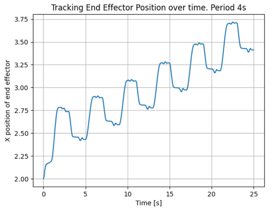
Figure 5. Simulated end‑effector x‑position versus time for a 4 s gait period.

Period of 2 seconds

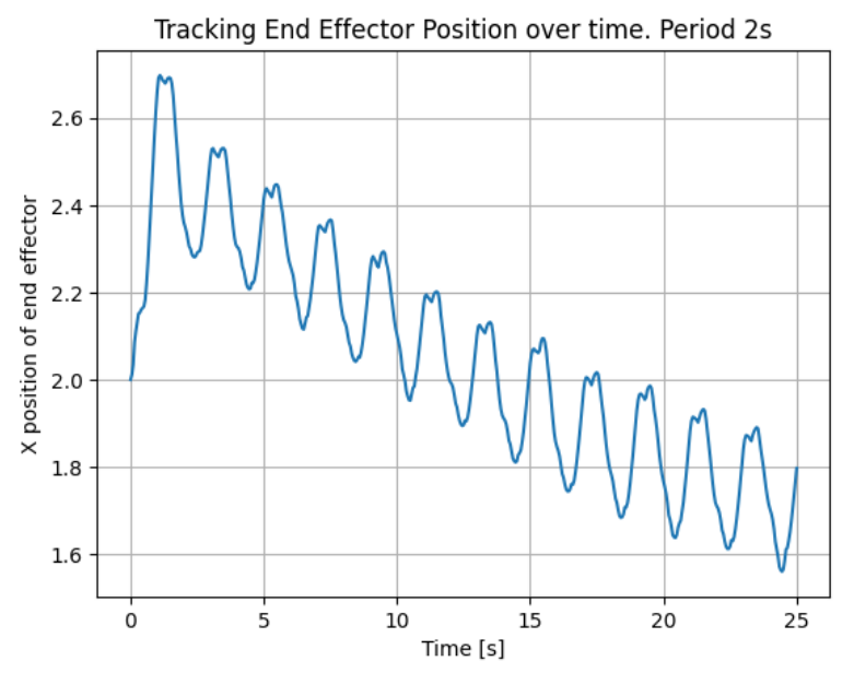
Figure 6. Simulated end‑effector x‑position versus time for a 2 s gait period.

Period of 1 second

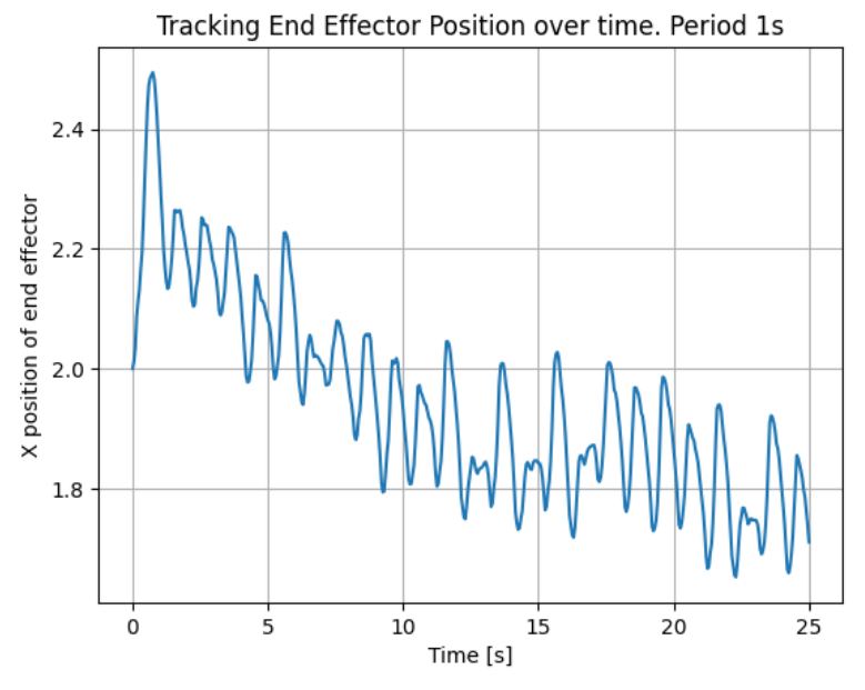
Figure 7. Simulated end‑effector x‑position versus time for a 1 s gait period.

Period of .5 seconds

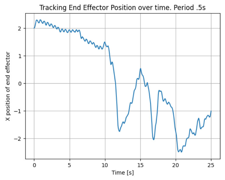
Figure 8. Simulated end‑effector x‑position versus time for a 0.5 s gait period.

Combination plot of all periods

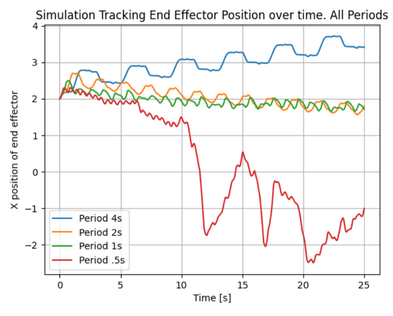
Figure 9. Simulated end‑effector trajectories for all gait periods overlaid, used to compare average forward speed and step quality as a function of gait period.

1.8 Sources of Error and Model Limitations

This section summarizes likely sources of discrepancy between the MuJoCo simulations and the experimental results, with emphasis on how modeling choices affect the timing study.

Geometry and mass properties
- Link bodies are represented as simple rectangular boxes, whereas the physical robot uses a folded triangular shell; this approximation shifts the true mass distribution and inertias.
- Wiring, servo housings, and 3D‑printed brackets are not modeled explicitly, further altering the effective mass and center of mass.
- Small scaling inconsistencies between CAD, cut patterns, and the MuJoCo geometry may change effective stride length and pad spacing.
Compliance modeling
- Each flexure is modeled as a single torsional spring–damper pair, while the real laminated hinges exhibit distributed bending, nonlinear stiffness, and possible hysteresis.
- The stiffness and damping parameters from Assignment 5 are applied uniformly to several joints; any joint‑to‑joint variation in the hardware is therefore not captured.
Contact and friction
- Pad and body friction coefficients in the XML are based on a single set of friction tests and may not match the friction experienced during the gait trials (for example, due to surface wear or contamination).
- The model assumes isotropic Coulomb friction with constant coefficients, whereas the physical pads may exhibit direction dependence and load‑dependent behavior.
- The measured friction ratio between pad and body is lower than the ideal design target, which can reduce anchoring robustness at shorter gait periods.
Actuator and control
- Position actuators in MuJoCo do not include explicit torque limits, backlash, or deadband, while the physical RC servos exhibit all of these effects.
- The fitted actuator gains \(k_{\text{motor}}\) and \(b_{\text{motor}}\) are approximate and do not fully reproduce servo dynamics at high command frequencies.
- Timing and phase offsets in the ESP32 control code, as well as servo‑to‑servo variability, lead to imperfect coordination between pads and body.
- In the current simulations, a persistent issue is incomplete motion at the central Sarrus hinge, especially for the 0.5 s gait period: the mid joint does not always reach its commanded extremes, and the desired lift–drag cycle is not fully realized. This limitation was not fully resolved within the project timeline and should be addressed in future model revisions.
Measurement and tracking
- Camera‑based tracking of the physical robot introduces noise due to limited frame rate, marker occlusion, and manual selection of tracking points.
- Small errors in coordinate calibration and time synchronization between video and control signals contribute additional uncertainty to the experimental displacement and speed estimates.

These limitations explain why the simulations tend to be more repeatable and slightly optimistic in speed compared with the hardware results, particularly at slower gait periods where real‑world slip, compliance losses, and servo saturation are more pronounced.

Here is a link to the .ipynb:

Inchworm

Inchworm Foldable Robotics

Dynamic MuJoCo Model and Simulation

1.1 Robot Overview and Objectives

1.2 Model Structure: Bodies, Joints, and Contacts

1.3 Compliance and Actuator Modeling

1.4 Sensing and Performance Metric Definition

1.5 MuJoCo XML Template

1.6 Python: Loading and Running a Single Simulation

Period of 2 seconds

Period of 1 second

Period of .5 seconds

1.7 Plotting Simulation Results

Period of 4 seconds

Period of 2 seconds

Period of 1 second

Period of .5 seconds

Combination plot of all periods

1.8 Sources of Error and Model Limitations